Regression task for predicting medical costs
Introduction
In this example, an exploratory data analysis will be performed, including an initial inspection of the set structure, studying the distributions of features and the target variable, identifying omissions, outliers and duplicates, as well as analyzing correlations between variables. At the next stage, regression models will be built and trained in order to predict the target variable and evaluate the quality of their work using appropriate metrics. Additionally, an analysis of the importance of the features will be performed, which will determine which of them make the greatest contribution to the predictions of the model and can be considered the most significant for the task under study.
Libraries must be installed
You must manually specify the paths where the project is located in order to go to the working directory, as well as install the necessary dependencies.
Before starting work, we will import all the necessary libraries.
!pip install -r /user/Demo_public/biomedical/predictionmeddata/requirements.txt
import pandas as pd
import matplotlib.pyplot as plt
import seaborn as sns
import numpy as np
from scipy.stats import randint, uniform, loguniform
from sklearn.model_selection import train_test_split, RandomizedSearchCV, KFold
from sklearn.linear_model import Lasso
from sklearn.metrics import mean_absolute_error, mean_squared_error, r2_score
from sklearn.ensemble import RandomForestRegressor
from catboost import CatBoostRegressor
We count the data and see what they are.
df = pd.read_csv("insurance.csv")
df.head(10)
Let's analyze the table:
- age — age
- sex — gender
- BMI — body mass index
- children — number of children
- smoker — smokes or not
- region — region of residence
- charges — medical expenses
Based on this table, we have features 1 through 6 - input data to the regression model, feature 7 - the target that needs to be predicted based on features 1-6.
EDA analysis
Let's check the table for gaps
df.info()
There are no passes. We see in the table 3 categorical features that will later be encoded for training the model, the rest of the features are numeric. You can also see that there are no gaps.
df.describe()
Statistics show that the average age of people is 39 years old with a deviation of 14, that is, it ranges from 25 to 53. It is also seen that bmi = 53 is present - this is the maximum value, which greatly exceeds the critical threshold. Maybe it's an outlier. It is also seen that half of people have a bmi of more than 30, meaning most suffer from the initial stages of obesity, and a quarter of clients have the last degree of obesity. The maximum cost is 63k conventional units (CU), which is very out of the picture (mean + 3sigma, mean -3sigma), perhaps this observation is also an outlier
Classical machine learning models cannot work with categorical features, that is, features that are not numbers. They need to be encoded into numbers. We use the One Hot Encoding technique
df_encode = pd.get_dummies(df, columns=["sex", "region", "smoker"])
df_encode = df_encode.drop('sex_female', axis=1)
df_encode = df_encode.drop('smoker_no', axis=1)
df_encode.head()
First, let's study the distribution of data. Let's build histograms for the signs
colors = ['blue', 'green', 'red', 'purple', 'orange']
fig, axes = plt.subplots(nrows=4, ncols=1,figsize=(7, 7))
axes = axes.flatten()
axes[0].hist(df["age"], bins=10, color=colors[0])
axes[0].set_title('Age')
axes[0].set_xlabel("Age of people")
axes[0].set_ylabel("Number of people")

axes[1].hist(df["bmi"], bins=10, color=colors[0])
axes[1].set_title('bmi')
axes[1].set_xlabel("bmi")
axes[1].set_ylabel("Number of people")

axes[2].hist(df["children"], bins=6, color=colors[0])
axes[2].set_title('Children')
axes[2].set_xlabel("Number of children")
axes[2].set_ylabel("Number of people")

axes[3].hist(df["charges"], bins=10, color=colors[0])
axes[3].set_title('Expenses')
axes[3].set_xlabel("People's expenses")
axes[3].set_ylabel("Number of people")
plt.subplots_adjust(hspace=0.6)
plt.tight_layout()
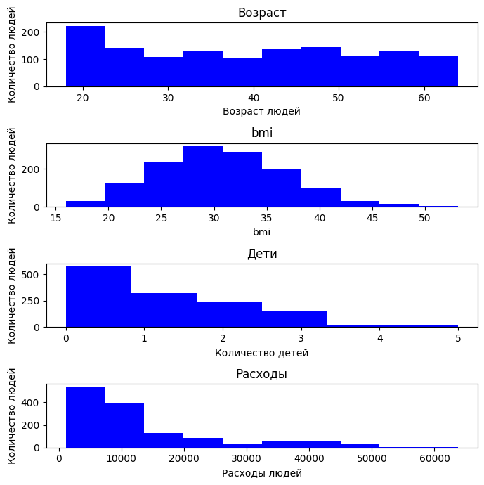
By age, it can be seen that the data in the sample is distributed fairly evenly: there are both young (from 18 years old) and elderly (up to 64 years old), but there are no noticeable distortions.
The BMI distribution has the appearance of a normal distribution, like a bell shifted to the right. Most people are in the range of 25 to 35, which corresponds to being overweight and obese. There are clients with very high BMI (>40).
In terms of the number of children, the distribution is sharply skewed: most clients do not have children.
It can be seen from the expenses that most people prefer to spend less than 30k units.
Next, we will analyze how one or another feature depends on each other. Consider the correlation of features. We will use the Spearman correlation, since it does not require the normality of the distribution.
spearman_corr = df_encode.corr(method='spearman')
spearman_corr['charges'].sort_values(ascending=False)
Based on the table above, we can conclude that smoking and age factors have a high correlation with expenses, that is, if a person smokes, then he has more expenses due to the need to spend on cigarettes. Similarly with age. Depending on the age, a person has different expenses. It can also be understood that the number of children does not greatly affect spending (you can see that most of those observed do not have children, so the correlation with spending is small), as well as the region of residence, gender and bmi.
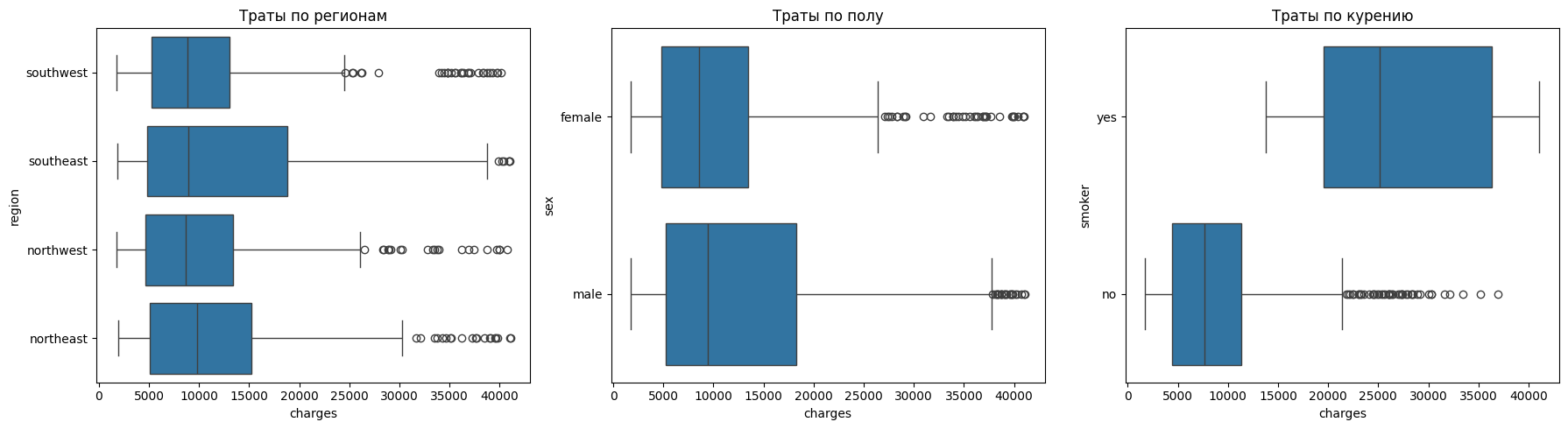
Let's see how categorical features affect spending.
fig, axes = plt.subplots(1, 3, figsize=(18, 5))
sns.boxplot(y="region", x="charges", data=df, ax=axes[0])
axes[0].set_title("Spending by region")

sns.boxplot(y="sex", x="charges", data=df, ax=axes[1])
axes[1].set_title("Spending by gender")

sns.boxplot(y="smoker", x="charges", data=df, ax=axes[2])
axes[2].set_title("Smoking expenses")

plt.tight_layout()
plt.show()
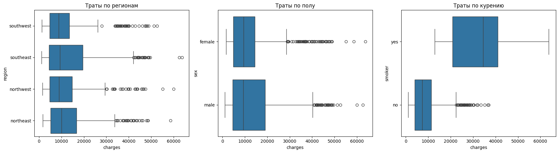
It can be seen from the regions that there are practically no differences in costs. Regions have similar distributions, and emissions are found everywhere.
There are also no noticeable differences in gender.
The situation with smoking is reversed. For non—smokers, the costs are less than 10 thousand, and for smokers - about 35 thousand. The spread among smokers is also much wider, which indicates that there are a large number of cases with extremely high costs.
plt.figure(figsize=(8,5))
sns.scatterplot(x="age", y="charges", hue="smoker", data=df, alpha=0.6)
plt.title("Dependence of expenses on age, taking into account smoking")
plt.xlabel("Age")
plt.ylabel("Expenses ")
plt.show()
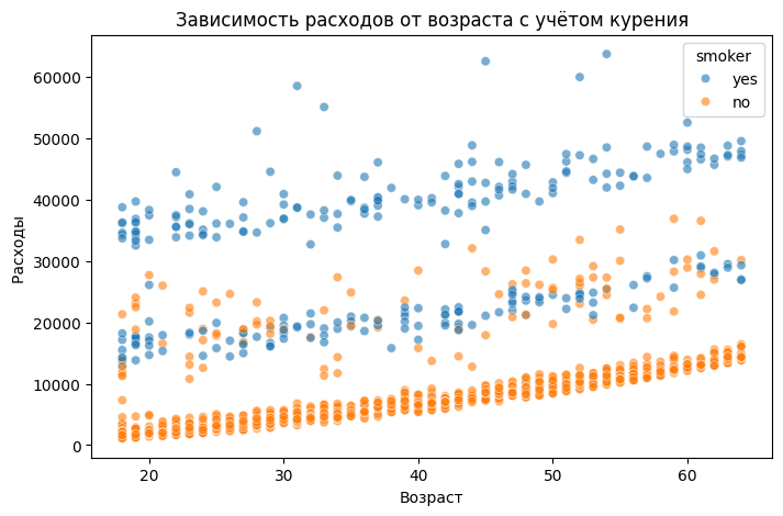
You can see that the costs increase linearly with age, that is, servicing older people is more expensive. It is also clear that there is a certain coefficient by which the dependence of expenses on age is shifted in the presence of the smoking factor.
df['bmi_group'] = pd.cut(df['bmi'], bins=[0, 25, 30, 100],
                         labels=['Standard', 'Overweight', 'Fatness'])
g = sns.FacetGrid(df, col="smoker", hue="bmi_group", height=5)
g.map(sns.scatterplot, "age", "charges", alpha=0.6).add_legend()
plt.show()
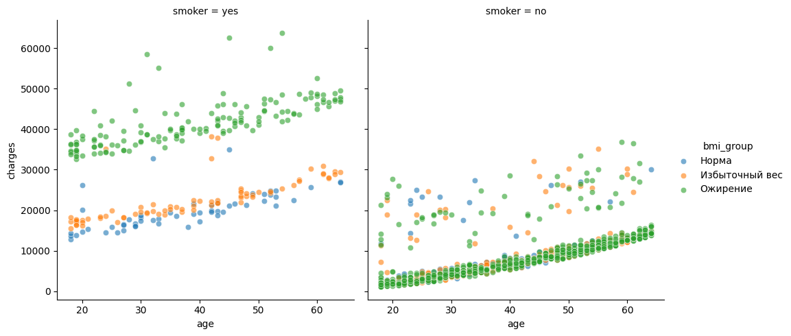
The following conclusions can be drawn from the graphs above:
For non-smokers, expenses increase with age, but generally remain within moderate limits. Even with obesity, the costs usually do not exceed 20-25 thousand. This suggests that without the smoking factor, the effect of weight is not so pronounced.
Two lines are clearly visible among smokers: one group of smokers spends on average about 20 thousand - people with normal weight or overweight, and the other group is consistently higher — about 35-50 thousand - these are obese smokers.
Let's check whether the number of children affects people's expenses.
plt.figure(figsize=(8,5))
sns.barplot(x="children", y="charges", data=df, estimator=lambda x: x.mean())
plt.title("Average expenses by number of children")
plt.xlabel("Number of children")
plt.ylabel("Average expenses")
plt.show()
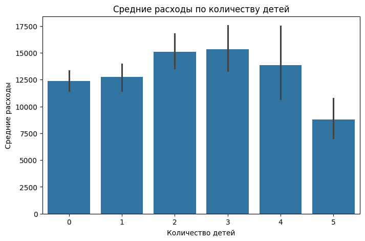
The number of children has virtually no effect on medical expenses. The only thing is when there are 2-3 children, the expenses are slightly higher than average
Let's look at the overall picture of the correlation of signs, draw a heat map, which is shown below.
sns.heatmap(df_encode.corr(method='spearman'), cmap="coolwarm", annot=False)
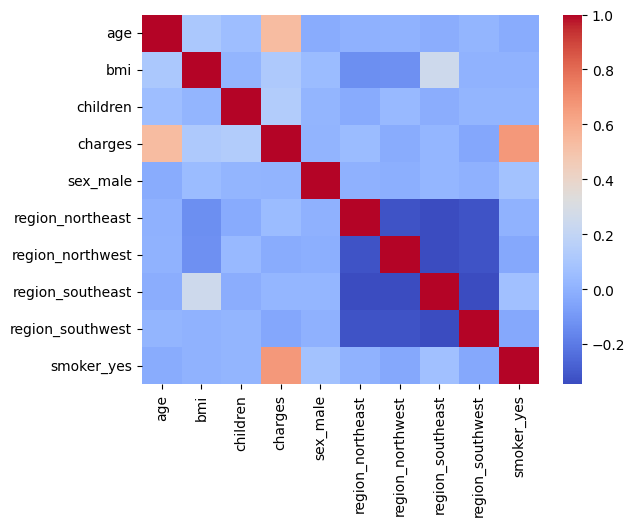
If you look at the correlation by signs, you can also see that there is a slight relationship between bmi and the region of residence, and in particular the "Southwest" region. That is, they have a more pronounced linear relationship.
Model training
The list of models that we will evaluate during training
- Linear Regression
- Random Forest
- CatBoost Regressor
Liner Regression (Lasso)
Let's create a table where we will record the results of model training.
Result_model = pd.DataFrame(columns=["Model", "MAE", "RMSE", "R2"])
For linear models, it is important to work correctly with categorical variables, which is why we encoded them using One Hot Encoding.
In the code below, y is our target variable, costs, and X is the features on which the model will be trained. The overall data set is divided into a test and a training set, so that after training the model, we can evaluate its generalizing ability on data that it has not yet encountered.
Metrics that we will use to evaluate the trained model:
- MAE is the average absolute error, it will show how much the model is wrong on average.
- RMSE is the root-mean-square error, large errors are more heavily penalized
- R2 is the coefficient of determination, which shows how well the model explains the "data
X = df_encode.drop("charges", axis=1)
y = df_encode["charges"]

X_train, X_test, y_train, y_test = train_test_split(X, y, test_size=0.2)
The first model will be Lasso. The code below provides training, calculation of metrics, and output of those features that the model considers less informative. However, even such signs can have a significant contribution.
lasso = Lasso(alpha=0.5)

lasso.fit(X_train, y_train)

y_pred_lasso = lasso.predict(X_test)

mae_lasso = mean_absolute_error(y_test, y_pred_lasso)
rmse_lasso = np.sqrt(mean_squared_error(y_test, y_pred_lasso))
r2_lasso = r2_score(y_test, y_pred_lasso)

print("Lasso Regression")
print("MAE:", mae_lasso)
print("RMSE:", rmse_lasso)
print("R²:", r2_lasso)

coef_lasso = pd.DataFrame({
    "Feature": X.columns,
    "Coefficient": lasso.coef_
}).sort_values(by="Coefficient", ascending=False)

print("Lasso Coefficients:")
print(coef_lasso)
Adding metric values to the table
row = pd.DataFrame({
    "Model": ["Lasso"],
    "MAE": [mae_lasso],
    "RMSE": [rmse_lasso],
    "R2": [r2_lasso]
})

Result_model = pd.concat([Result_model, row])
Random Forest
The next model will be a random forest. The principle is the same, we train, we test, we look at the importance of signs
rf = RandomForestRegressor(
    n_estimators=100,
    max_depth=4,
    min_samples_split = 20,
    min_samples_leaf = 20
)

rf.fit(X_train, y_train)

y_pred_rf = rf.predict(X_test)

mae_rf = mean_absolute_error(y_test, y_pred_rf)
rmse_rf = np.sqrt(mean_squared_error(y_test, y_pred_rf))
r2_rf = r2_score(y_test, y_pred_rf)

print("Random Forest")
print("MAE:", mae_rf)
print("RMSE:", rmse_rf)
print("R²:", r2_rf)

importances = pd.DataFrame({
    "Feature": X.columns,
    "Importance": rf.feature_importances_
}).sort_values(by="Importance", ascending=False)

print("\The importance of signs:")
print(importances)
Adding metrics to the table
row = pd.DataFrame({
    "Model": ["Random Forest"],
    "MAE": [mae_rf],
    "RMSE": [rmse_rf],
    "R2": [r2_rf]
})

Result_model = pd.concat([Result_model, row])
It can be seen that the metrics of the random forest model are much better than those of the linear model.
CatBoost Regressor
The next model is the gradient boosting model from the CatBosot package. Let's go through the same pipeline as with the models above.
cat_features = ["smoker", "sex", "region"]
feature_cols = [c for c in df.columns if c not in ["charges"]]


cat = CatBoostRegressor(
    iterations=1000,
    depth=6,
    learning_rate=0.01,
    verbose=100, random_state=42
)

X = df[feature_cols]
y = df["charges"]

X_train, X_test, y_train, y_test = train_test_split(X, y, test_size=0.3, random_state=42)

cat.fit(X_train, y_train, cat_features=cat_features, eval_set=(X_test, y_test), verbose=100)

y_pred_cat = cat.predict(X_test)

mae_cat1 = mean_absolute_error(y_test, y_pred_cat)
rmse_cat1 = np.sqrt(mean_squared_error(y_test, y_pred_cat))
r2_cat1 = r2_score(y_test, y_pred_cat)

feature_importance = cat.get_feature_importance(prettified=True)
print(feature_importance)

print("CatBoost")
print("MAE:", mae_cat1)
print("RMSE:", rmse_cat1)
print("R²:", r2_cat1)
Adding metrics to the table
row = pd.DataFrame({
    "Model": ["CatBoostRegressor 1ver"],
    "MAE": [mae_cat1],
    "RMSE": [rmse_cat1],
    "R2": [r2_cat1]
})

Result_model = pd.concat([Result_model, row])
Next, we will try to select more optimal hyperparameters for the gradient boosting model. Here, three metrics that I described above will be taken into account at once.
We will search for hyperparameters by randomly selecting the parameters and their ranges that the model works with.
scoring = {
    "mae": "neg_mean_absolute_error",
    "rmse": "neg_root_mean_squared_error",
    "r2": "r2",
}

cat_base = CatBoostRegressor(
    verbose=False,
    random_state=42,
    task_type="GPU",
    devices="0"
)

param_distributions = {
    "iterations": randint(300, 1000),
    "depth": randint(4, 8),
    "learning_rate": loguniform(1e-3, 3e-1),
    "l2_leaf_reg": loguniform(1e-2, 1e2),
    "bagging_temperature": uniform(0.0, 1.0),
    "random_strength": loguniform(1e-3, 10),
    "grow_policy": ["SymmetricTree", "Depthwise"],
    "border_count": randint(32, 128),
    "leaf_estimation_iterations": randint(1, 3)
}

rs = RandomizedSearchCV(
    estimator=cat_base,
    param_distributions=param_distributions,
    n_iter=20,
    scoring=scoring,
    cv=KFold(n_splits=5, shuffle=True, random_state=42),
    n_jobs=1,
    random_state=42,
    refit=False
)


rs.fit(X_train, y_train, cat_features=cat_features)
Next, we will find the best result among all the metrics. In our case, the coefficient of determination showed generally the best figures for all metrics.
cv = rs.cv_results_
best_idx = np.argmax(cv["mean_test_r2"])
best_params = cv["params"][best_idx]
print("Best configuration by r2:", best_params)
Using the obtained hyperparameters, we will train the model
best_cat = CatBoostRegressor(
    verbose=False, random_state=42, task_type="GPU", devices="0", **best_params
)
best_cat.fit(X_train, y_train, cat_features=cat_features)

y_pred = best_cat.predict(X_test)

mae  = mean_absolute_error(y_test, y_pred)
rmse = np.sqrt(mean_squared_error(y_test, y_pred))
r2   = r2_score(y_test, y_pred)

print("MAE:", mae)
print("RMSE:", rmse)
print("R²:", r2)

fi = best_cat.get_feature_importance(prettified=True)
print(fi)
And we will also add the calculated metrics to the table.
row = pd.DataFrame({
    "Model": ["CatBoostRegressor 2ver"],
    "MAE": [mae],
    "RMSE": [rmse],
    "R2": [r2]
})

Result_model = pd.concat([Result_model, row])
Let's do Feature Engineering by creating new features from existing ones. In our case, we divide the age into decades, divide people with children into groups, and also divide the bmi index into classes (that is, by intervals).
df = pd.read_csv("insurance.csv")
df["age_decade"] = (df["age"] // 10).astype(int).astype("category")
df["children_bucket"] = pd.cut(df["children"], [-1,0,2,99], labels=["0","1-2","3+"])
df["obesity_class"] = pd.cut(df["bmi"],
    [0,18.5,25,30,35,40,1e3], labels=["Under","Normal","Over","Ob1","Ob2", "Ob3"])
After that, we will conduct the same pipeline for training the basic model.
cat_features = ["smoker", "sex", "region", "obesity_class", "age_decade", "children_bucket"]
feature_cols = [c for c in df.columns if c not in ["charges"]]


cat = CatBoostRegressor(
    iterations=2000,
    depth=6,
    learning_rate=0.01,
    verbose=100, random_state=42
)

X = df[feature_cols]
y = df["charges"]

X_train, X_test, y_train, y_test = train_test_split(X, y, test_size=0.2, random_state=42)

cat.fit(X_train, y_train, cat_features=cat_features, eval_set=(X_test, y_test), verbose=100)

y_pred_cat = cat.predict(X_test)

mae_cat = mean_absolute_error(y_test, y_pred_cat)
rmse_cat = np.sqrt(mean_squared_error(y_test, y_pred_cat))
r2_cat = r2_score(y_test, y_pred_cat)

feature_importance = cat.get_feature_importance(prettified=True)
print(feature_importance)

print("CatBoost")
print("MAE:", mae_cat)
print("RMSE:", rmse_cat)
print("R²:", r2_cat)
Well, let's write down the metrics in the table.
row = pd.DataFrame({
    "Model": ["CatBoostRegressor 3ver"],
    "MAE": [mae_cat],
    "RMSE": [rmse_cat],
    "R2": [r2_cat]
})

Result_model = pd.concat([Result_model, row])
Next, let's check how the model with the best parameters, which were found through a random search, behaves on a dataset with new features.
cat_features = ["smoker", "sex", "region", "obesity_class", "age_decade", "children_bucket"]
feature_cols = [c for c in df.columns if c not in ["charges"]]


best_cat = CatBoostRegressor(
    verbose=False, random_state=42, task_type="GPU", devices="0", **best_params
)

X = df[feature_cols]
y = df["charges"]

X_train, X_test, y_train, y_test = train_test_split(X, y, test_size=0.15, random_state=42)

cat.fit(X_train, y_train, cat_features=cat_features, eval_set=(X_test, y_test), verbose=100)

y_pred_cat = cat.predict(X_test)

mae_cat = mean_absolute_error(y_test, y_pred_cat)
rmse_cat = np.sqrt(mean_squared_error(y_test, y_pred_cat))
r2_cat = r2_score(y_test, y_pred_cat)

feature_importance = cat.get_feature_importance(prettified=True)
print(feature_importance)

print("CatBoost")
print("MAE:", mae_cat)
print("RMSE:", rmse_cat)
print("R²:", r2_cat)
As usual, we record the results in a table.
row = pd.DataFrame({
    "Model": ["CatBoostRegressor 4ver"],
    "MAE": [mae_cat],
    "RMSE": [rmse_cat],
    "R2": [r2_cat]
})

Result_model = pd.concat([Result_model, row])
Let's conduct an experiment. We'll find the outliers and delete them. Let's check how the gradient booster model behaves.
In this case, we are deleting data that can greatly distort the picture for the model and spoil the metrics, of course.
We delete the following data:
0.05 is the quantile— the value below which 5% of observations are located.
0.95 is the quantile value above which 5% of observations are found.
df = pd.read_csv("insurance.csv")

numeric_cols = df.select_dtypes(include=[np.number]).columns

low = df[numeric_cols].quantile(0.05)
high = df[numeric_cols].quantile(0.95)

df_no_outliers = df[~((df[numeric_cols] < low) | (df[numeric_cols] > high)).any(axis=1)]
We will display information about the dataset
df_no_outliers.info()
It can be seen that about 300 copies of the data have been deleted. In this case, we lose 20 percent of all information, which is not recommended, but we look at how these 20 percent affect the final prediction of the model.
Let's build the boxplots that were built in the paragraph above and estimate the distribution of the data.
fig, axes = plt.subplots(1, 3, figsize=(18, 5))
sns.boxplot(y="region", x="charges", data=df_no_outliers, ax=axes[0])
axes[0].set_title("Spending by region")

sns.boxplot(y="sex", x="charges", data=df_no_outliers, ax=axes[1])
axes[1].set_title("Spending by gender")

sns.boxplot(y="smoker", x="charges", data=df_no_outliers, ax=axes[2])
axes[2].set_title("Smoking expenses")

plt.tight_layout()
plt.show()
It can be seen that there are slightly fewer emissions
Next, we will train the gradient boosting model on the cropped dataset and check the metrics
cat_features = ["smoker", "sex", "region"]
feature_cols = [c for c in df.columns if c not in ["charges"]]


cat = CatBoostRegressor(
    iterations=2700,
    depth=9,
    learning_rate=0.002,
    verbose=100, random_state=42
)

X = df_no_outliers[feature_cols]
y = df_no_outliers["charges"]

X_train, X_test, y_train, y_test = train_test_split(X, y, test_size=0.15, random_state=42)

cat.fit(X_train, y_train, cat_features=cat_features, eval_set=(X_test, y_test), verbose=100)

y_pred_cat = cat.predict(X_test)

mae_cat = mean_absolute_error(y_test, y_pred_cat)
rmse_cat = np.sqrt(mean_squared_error(y_test, y_pred_cat))
r2_cat = r2_score(y_test, y_pred_cat)

feature_importance = cat.get_feature_importance(prettified=True)
print(feature_importance)

print("CatBoost")
print("MAE:", mae_cat)
print("RMSE:", rmse_cat)
print("R²:", r2_cat)
Let's put everything on the tablet
row = pd.DataFrame({
    "Model": ["CatBoostRegressor 5ver"],
    "MAE": [mae_cat],
    "RMSE": [rmse_cat],
    "R2": [r2_cat]
})

Result_model = pd.concat([Result_model, row], ignore_index=True)
Let's evaluate the results
Result_model
It can be seen from the table below that the best values of the R2 metric were shown by the Random Forest and gradient boosting models (version 5). However, it should be borne in mind that the gradient boosting model was trained on transformed data, where potential outliers were removed (even if such clients may actually occur in the sample). At the same time, the Random Forest model demonstrates a higher R2 value on the initial dataset, but its RMSE and MAE indicators are worse. This indicates the presence in the initial data of observations with costs significantly higher than the average level. So, with an average value of about 20 thousand units, there are cases with expenses of about 60 thousand units. Such extreme values increase the errors in the absolute metrics of Random Forest. In contrast, the gradient boosting model, trained without outliers, showed lower MAE and RMSE errors.
Thus, among all the trained models, we will consider the one that has the lowest metrics in total to be the best.
In our case, this is gradient boosting version 5.
What factors influence target the most?
Let's evaluate the importance of the signs with 2 spokes:
- Importance based on EDA
- Importance gained with the help of models
Importance based on EDA
Let's consider all the signs separately
Smoking (smoker)
The most significant factor. The correlation coefficient between smoking and expenses is 0.66, which indicates a strong relationship.
The graphs show that smokers have significantly higher expenses than non-smokers.
The scatter plot also shows that even with the same age and BMI, smokers have significantly higher costs.
Smoking dramatically increases health risks (heart disease, lung disease, cancer), which leads to higher costs.
Age (age)
Age comes in second place in terms of influence (correlation 0.53).
The graphs show that the older a person is, the higher the costs.
This is especially noticeable for smokers: as they age, their expenses increase, and it looks a bit like an exponential dependence.
The reason is that with age, the likelihood of chronic diseases and seeking medical help increases.
The presence of children
The correlation is weak (0.13), but still positive.
Families with 2-3 children have higher expenses on average than those without children or with one child.
However, with 5 children, average expenses decrease — this may be due to the characteristics of the sample.
The reason is that having children increases health costs
Body Mass Index (BMI)
The correlation with expenses is weak (0.11), but in combination with other factors, BMI plays a role.
The graphs show that obese people have higher expenses, especially if they smoke.
At the same time, obesity without smoking does not always lead to a sharp increase in costs.
The reason is that obesity is associated with the risks of diabetes and cardiovascular diseases, but these effects are enhanced by other risk factors.
Gender and region (sex, region)
There is no noticeable effect by gender or region.
Correlations are close to zero.
The distribution of expenses is almost the same for men and women, as well as for different regions.
The reason is that insurance rates and medicine do not depend on the region of residence or gender in this sample.
Importance obtained with the help of models
We will see a similar picture of importance if we look at which features have more and which have less weight after training the model.
So, for example, for the Random Forest model, the coefficients of importance of features after training:
-
smoker_yes 0.700647 -
bmi 0.175183 -
age 0.115571
It can be seen that during the EDA it was also found that these very signs are of high importance.
For example, for two models of gradient boosting, it was these features that were important, just with different coefficients.:
-
smoker -
bmi -
age
Thus, it can be unequivocally concluded that the most significant signs are the smoking factor, the bmi index, and age.
Conclusion
In the example, an exploratory data analysis was performed, regression models were trained, and the most significant features affecting the target variable were identified.